Journal Article in SIAM Journal on Applied Dynamical Systems
Physics-based and first-principles models pervade the engineering and physical sciences, allowing for the ability to model the dynamics of complex systems with a prescribed accuracy. The approximations used in deriving governing equations often result in discrepancies between the model and sensor-based measurements of the system, revealing the approximate nature of the equations and/or the signal-to-noise ratio of the sensor itself. In modern dynamical systems, such discrepancies between model and measurement can lead to poor quantification, often undermining the ability to produce accurate and precise control algorithms.
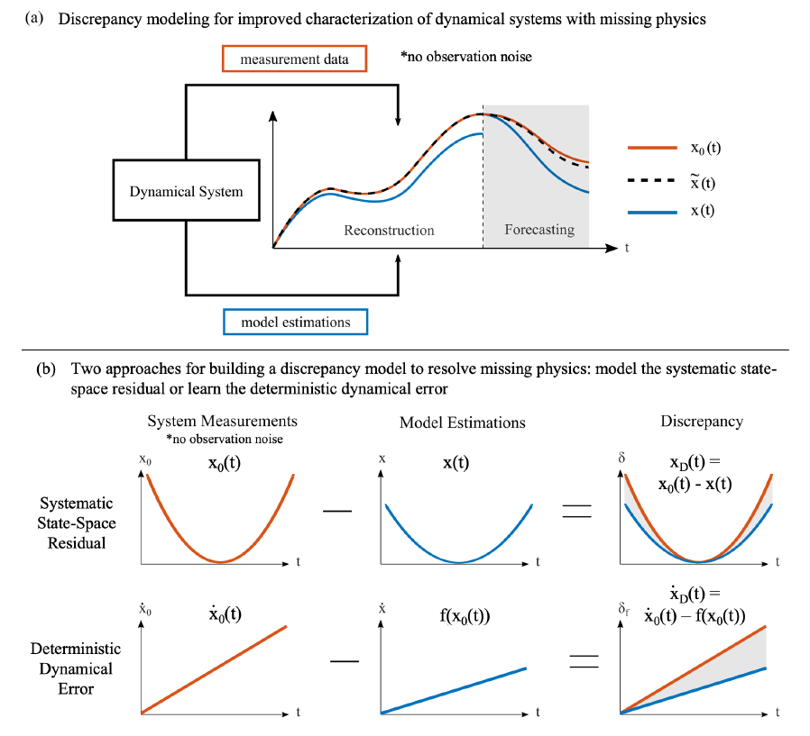
Aim: Introduce a discrepancy modeling framework to identify the missing physics and resolve the model-measurement mismatch with two distinct approaches: (i) by learning a model for the evolution of systematic state-space residual, and (ii) by discovering a model for the deterministic dynamical error. Regardless of approach, a common suite of data-driven model discovery methods can be used.
Method: Specifically, we use four fundamentally different methods to demonstrate the mathematical implementations of discrepancy modeling: (i) the sparse identification of nonlinear dynamics (SINDy), (ii) dynamic mode decomposition (DMD), (iii) Gaussian process regression (GPR), and (iv) neural networks (NN). The choice of method depends on one’s intent (e.g., mechanistic interpretability) for discrepancy modeling, sensor measurement characteristics (e.g., quantity, quality, resolution), and constraints imposed by practical applications (e.g., state- or dynamical-space operability).
Results: We demonstrate the utility and suitability for both discrepancy modeling approaches using the suite of data-driven modeling methods on three continuous dynamical systems under varying signal-to-noise ratios. Finally, we emphasize structural shortcomings of each discrepancy modeling approach depending on error type.
Interpretation: In summary, if the true dynamics are unknown (i.e., an imperfect model), one should learn a discrepancy model of the missing physics in the dynamical space. Yet, if the true dynamics are known yet model-measurement mismatch still exists, one should learn a discrepancy model in the state space.